require(pacman)
p_load(tidytuesdayR, magick, trashpanda, tidyverse, janitor, tidytext, slider, here, TTR, sf, rnaturalearth, rnaturalearthdata, patchwork)Scottish Munros
geography
maps
Mountains in Scotland
Load Packages
Load Data
tuesdata <- tidytuesdayR::tt_load('2025-08-19')
scottish_munros <- tuesdata$scottish_munros
Plot
# Get UK countries (scotland, england, etc.) from Natural Earth
uk <- ne_countries(country = "United Kingdom", scale = "medium", returnclass = "sf")
# Transform UK shapefile to British National Grid
uk_bng <- st_transform(uk, crs = 27700)
# Get rivers and lakes
rivers <- ne_download(scale = "medium", type = "rivers_lake_centerlines", category = "physical", returnclass = "sf")
lakes <- ne_download(scale = "medium", type = "lakes", category = "physical", returnclass = "sf")
rivers_bng <- st_transform(rivers, crs = 27700)
lakes_bng <- st_transform(lakes, crs = 27700)
# Get major cities
cities <- ne_download(scale = "medium", type = "populated_places", category = "cultural", returnclass = "sf")
cities_bng <- st_transform(cities, crs = 27700)
# Make sf object with British National Grid CRS
df_sf <- st_as_sf(scottish_munros |> drop_na(xcoord, ycoord), coords = c("xcoord", "ycoord"), crs = 27700)
density <- ggplot() +
geom_sf(data = lakes_bng, fill = "lightblue", color = NA) +
geom_sf(data = rivers_bng, color = "blue", size = 0.5) +
geom_sf(data = uk_bng, fill = NA, color = "black", size = 0.7) +
stat_density_2d(
data = df_sf,
aes(x = st_coordinates(df_sf)[,1], y = st_coordinates(df_sf)[,2], fill = after_stat(level * 1e9)),
geom = "polygon",
alpha = 0.4,
color = NA,
h = c(40000, 40000)
) +
scale_fill_viridis_c(option = "magma", name = "2D Kernel Density (x1e9)") +
coord_sf(crs = 27700,
xlim = c(0, 470000),
ylim = c(530000, 1200000)) +
theme_void() +
theme(
panel.border = element_rect(color = "black", fill = NA, size = 1),
panel.background = element_rect(fill = "white"),
legend.position = "bottom",
legend.title = element_text(vjust = 0.5, size = 25, margin = margin(r = 8)),
)
points <- ggplot() +
geom_sf(data = lakes_bng, fill = "lightblue", color = NA) +
geom_sf(data = rivers_bng, color = "blue", size = 0.5) +
geom_sf(data = uk_bng, fill = NA, color = "black", size = 0.7) +
scale_fill_viridis_c(option = "magma", name = "Density") +
geom_sf(
data = df_sf,
aes(color = Height_m, size = Height_m),
alpha = 0.8) +
scale_color_viridis_c(option = "plasma", name = "Height (m)", label = add_commas) +
scale_size_continuous(range = c(1,5), guide = "none") +
coord_sf(crs = 27700,
xlim = c(0, 470000),
ylim = c(530000, 1200000)) +
theme_void() +
theme(
panel.border = element_rect(color = "black", fill = NA, size = 1),
panel.background = element_rect(fill = "white"),
legend.position = "bottom",
legend.title = element_text(vjust = 0.5, size = 25, margin = margin(r = 20)))
plot <- points + density +
plot_annotation(
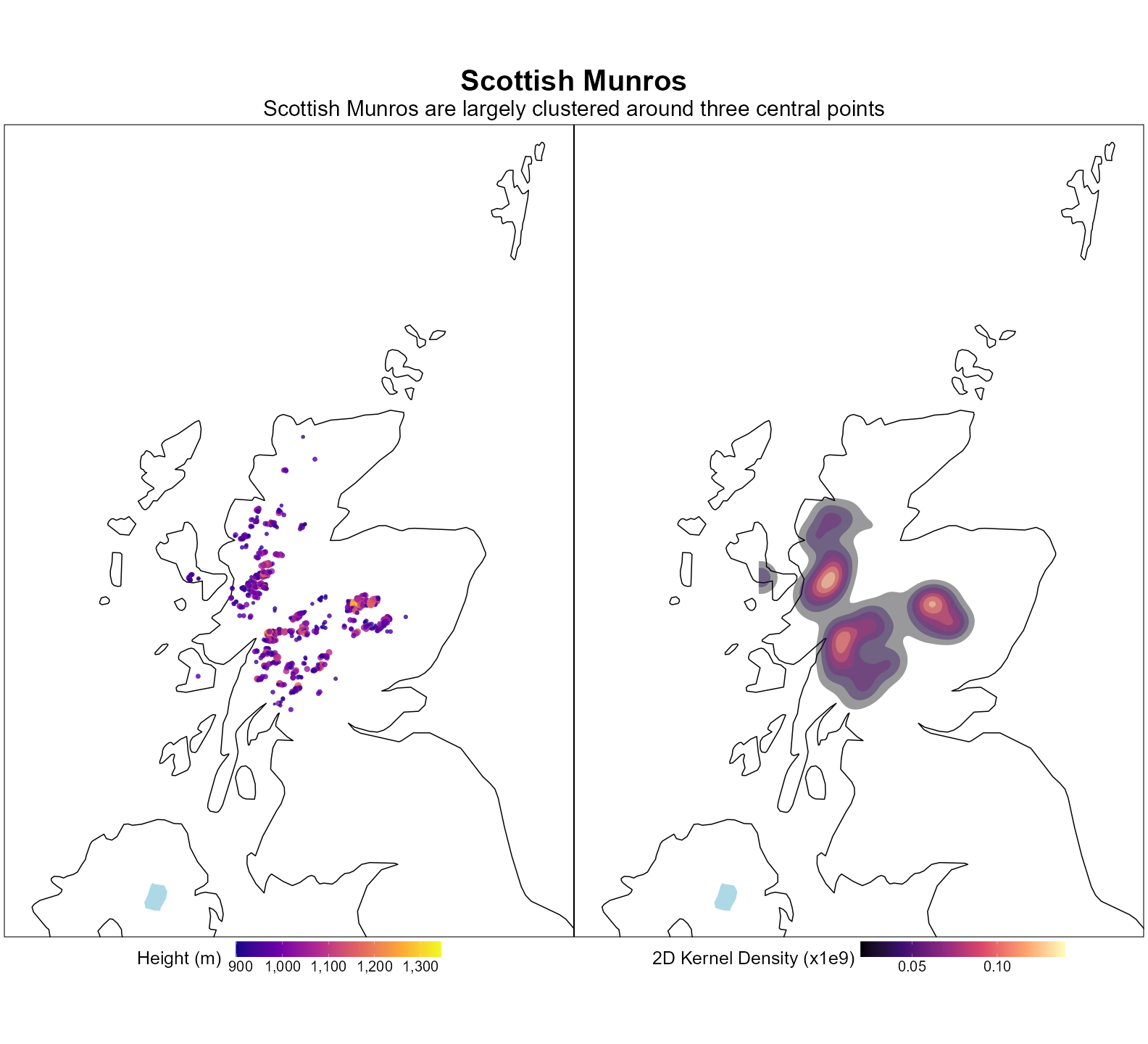
title = "Scottish Munros",
subtitle = "Scottish Munros are largely clustered around three central points"
) &
theme(legend.key.width = unit(2, "cm"),
legend.key.size = unit(1.5, "lines"),
legend.text = element_text(size = 20),
plot.title = element_text(face = "bold", hjust = 0.5, size = 40),
plot.subtitle = element_text(hjust = 0.5, size = 30))
# Save and display images
current_dir <- dirname(knitr::current_input())
plot_name <- "scottish_munros.png"
ggsave(plot = plot,
dpi = "screen",
width = 22,
height = 20,
device = ragg::agg_png,
filename = file.path(current_dir, plot_name))
# Read the big plot
img <- image_read(file.path(current_dir, plot_name))
# Force 16:9 aspect ratio with minimal padding
# Target size: 1200x675 px (16:9)
img_card <- image_scale(img, "1200x675") # scale to fit inside 16:9
img_card <- image_extent(
img_card,
geometry = "1200x675",
gravity = "center"
)
# Save as card preview
image_write(img_card, path = file.path(current_dir, "preview.png"))
knitr::include_graphics(
file.path(current_dir, plot_name)
)
References
trashpanda::cite_packages(format = "rmd")Pedersen T (2025). patchwork: The Composer of Plots. doi:10.32614/CRAN.package.patchwork https://doi.org/10.32614/CRAN.package.patchwork, R package version 1.3.2, https://CRAN.R-project.org/package=patchwork.
South A, Michael S, Massicotte P (2024). rnaturalearthdata: World Vector Map Data from Natural Earth Used in ‘rnaturalearth’. doi:10.32614/CRAN.package.rnaturalearthdata https://doi.org/10.32614/CRAN.package.rnaturalearthdata, R package version 1.0.0, https://CRAN.R-project.org/package=rnaturalearthdata.
Massicotte P, South A (2026). rnaturalearth: World Map Data from Natural Earth. doi:10.32614/CRAN.package.rnaturalearth https://doi.org/10.32614/CRAN.package.rnaturalearth, R package version 1.2.0, https://CRAN.R-project.org/package=rnaturalearth.
Pebesma E, Bivand R (2023). Spatial Data Science: With applications in R. Chapman and Hall/CRC. doi:10.1201/9780429459016 https://doi.org/10.1201/9780429459016, https://r-spatial.org/book/.
Pebesma E (2018). “Simple Features for R: Standardized Support for Spatial Vector Data.” The R Journal, 10(1), 439-446. doi:10.32614/RJ-2018-009 https://doi.org/10.32614/RJ-2018-009, https://doi.org/10.32614/RJ-2018-009.
Ulrich J (2023). TTR: Technical Trading Rules. doi:10.32614/CRAN.package.TTR https://doi.org/10.32614/CRAN.package.TTR, R package version 0.24.4, https://CRAN.R-project.org/package=TTR.
Müller K (2025). here: A Simpler Way to Find Your Files. doi:10.32614/CRAN.package.here https://doi.org/10.32614/CRAN.package.here, R package version 1.0.2, https://CRAN.R-project.org/package=here.
Vaughan D (2025). slider: Sliding Window Functions. doi:10.32614/CRAN.package.slider https://doi.org/10.32614/CRAN.package.slider, R package version 0.3.3, https://CRAN.R-project.org/package=slider.
Silge J, Robinson D (2016). “tidytext: Text Mining and Analysis Using Tidy Data Principles in R.” JOSS, 1(3). doi:10.21105/joss.00037 https://doi.org/10.21105/joss.00037, http://dx.doi.org/10.21105/joss.00037.
Firke S (2024). janitor: Simple Tools for Examining and Cleaning Dirty Data. doi:10.32614/CRAN.package.janitor https://doi.org/10.32614/CRAN.package.janitor, R package version 2.2.1, https://CRAN.R-project.org/package=janitor.
Grolemund G, Wickham H (2011). “Dates and Times Made Easy with lubridate.” Journal of Statistical Software, 40(3), 1-25. https://www.jstatsoft.org/v40/i03/.
Wickham H (2025). forcats: Tools for Working with Categorical Variables (Factors). doi:10.32614/CRAN.package.forcats https://doi.org/10.32614/CRAN.package.forcats, R package version 1.0.1, https://CRAN.R-project.org/package=forcats.
Wickham H (2025). stringr: Simple, Consistent Wrappers for Common String Operations. doi:10.32614/CRAN.package.stringr https://doi.org/10.32614/CRAN.package.stringr, R package version 1.6.0, https://CRAN.R-project.org/package=stringr.
Wickham H, François R, Henry L, Müller K, Vaughan D (2023). dplyr: A Grammar of Data Manipulation. doi:10.32614/CRAN.package.dplyr https://doi.org/10.32614/CRAN.package.dplyr, R package version 1.1.4, https://CRAN.R-project.org/package=dplyr.
Wickham H, Henry L (2026). purrr: Functional Programming Tools. doi:10.32614/CRAN.package.purrr https://doi.org/10.32614/CRAN.package.purrr, R package version 1.2.1, https://CRAN.R-project.org/package=purrr.
Wickham H, Hester J, Bryan J (2025). readr: Read Rectangular Text Data. doi:10.32614/CRAN.package.readr https://doi.org/10.32614/CRAN.package.readr, R package version 2.1.6, https://CRAN.R-project.org/package=readr.
Wickham H, Vaughan D, Girlich M (2025). tidyr: Tidy Messy Data. doi:10.32614/CRAN.package.tidyr https://doi.org/10.32614/CRAN.package.tidyr, R package version 1.3.2, https://CRAN.R-project.org/package=tidyr.
Müller K, Wickham H (2026). tibble: Simple Data Frames. doi:10.32614/CRAN.package.tibble https://doi.org/10.32614/CRAN.package.tibble, R package version 3.3.1, https://CRAN.R-project.org/package=tibble.
Wickham H (2016). ggplot2: Elegant Graphics for Data Analysis. Springer-Verlag New York. ISBN 978-3-319-24277-4, https://ggplot2.tidyverse.org.
Wickham H, Averick M, Bryan J, Chang W, McGowan LD, François R, Grolemund G, Hayes A, Henry L, Hester J, Kuhn M, Pedersen TL, Miller E, Bache SM, Müller K, Ooms J, Robinson D, Seidel DP, Spinu V, Takahashi K, Vaughan D, Wilke C, Woo K, Yutani H (2019). “Welcome to the tidyverse.” Journal of Open Source Software, 4(43), 1686. doi:10.21105/joss.01686 https://doi.org/10.21105/joss.01686.
Baril C (????). trashpanda: Cole’s Personal Collection of R Functions, Themes, and Palettes. R package version 0.0.1, https://colebaril.github.io/trashpanda/.
Ooms J (2025). magick: Advanced Graphics and Image-Processing in R. doi:10.32614/CRAN.package.magick https://doi.org/10.32614/CRAN.package.magick, R package version 2.9.0, https://CRAN.R-project.org/package=magick.
Harmon J, Hughes E (2025). tidytuesdayR: Access the Weekly ‘TidyTuesday’ Project Dataset. doi:10.32614/CRAN.package.tidytuesdayR https://doi.org/10.32614/CRAN.package.tidytuesdayR, R package version 1.2.1, https://CRAN.R-project.org/package=tidytuesdayR.
Rinker TW, Kurkiewicz D (2018). pacman: Package Management for R. version 0.5.0, http://github.com/trinker/pacman.